Basic functions¶

Drawing a point in a map¶

Drawing a point in a map is usually done using the plot method:

from mpl_toolkits.basemap import Basemap
import matplotlib.pyplot as plt

map = Basemap(projection='ortho', 
              lat_0=0, lon_0=0)

map.drawmapboundary(fill_color='aqua')
map.fillcontinents(color='coral',lake_color='aqua')
map.drawcoastlines()

x, y = map(0, 0)

map.plot(x, y, marker='D',color='m')

plt.show()

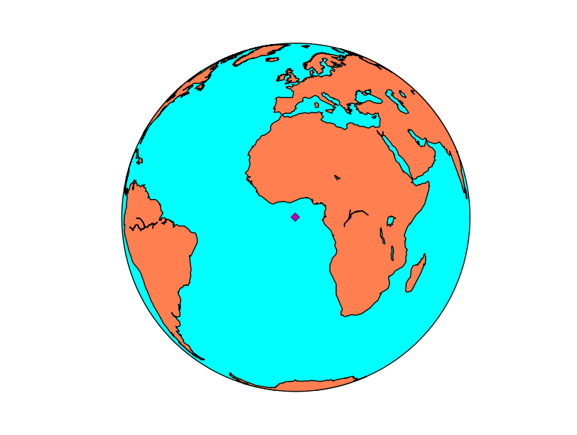
Use the Basemap instance to calculate the position of the point in the map coordinates when you have the longitude and latitude of the point
- If latlon keyword is set to True, x,y are interpreted as longitude and latitude in degrees. Won’t work in old basemap versions
The plot method needs the x and y position in the map coordinates, the marker and the color
- By default, the marker is a point. This page explains all the options
- By default, the color is black (k). This page explains all the color options

If you have more than one point, you may prefer the scatter method. Passing an array of point into the plot method creates a line connecting them, which may be interesting, but is not a point cloud:

from mpl_toolkits.basemap import Basemap
import matplotlib.pyplot as plt

map = Basemap(projection='ortho', 
              lat_0=0, lon_0=0)

map.drawmapboundary(fill_color='aqua')
map.fillcontinents(color='coral',lake_color='aqua')
map.drawcoastlines()

lons = [0, 10, -20, -20]
lats = [0, -10, 40, -20]

x, y = map(lons, lats)

map.scatter(x, y, marker='D',color='m')

plt.show()

Remember that calling the Basemap instance can be done with lists, so the coordinate transformation is done at once
The format options in the scatter method are the same as in plot

Plotting raster data¶

There are two main methods for plotting a raster, contour/contourf, that plots contour lines or filled contour lines (isobands) and pcolor/pcolormesh, that creates a pseudo-color plot.

contourf¶

from mpl_toolkits.basemap import Basemap
import matplotlib.pyplot as plt
from osgeo import gdal
from numpy import linspace
from numpy import meshgrid

map = Basemap(projection='tmerc', 
              lat_0=0, lon_0=3,
              llcrnrlon=1.819757266426611, 
              llcrnrlat=41.583851612359275, 
              urcrnrlon=1.841589961763497, 
              urcrnrlat=41.598674173123)

ds = gdal.Open("../sample_files/dem.tiff")
data = ds.ReadAsArray()

x = linspace(0, map.urcrnrx, data.shape[1])
y = linspace(0, map.urcrnry, data.shape[0])

xx, yy = meshgrid(x, y)

map.contourf(xx, yy, data)

plt.show()

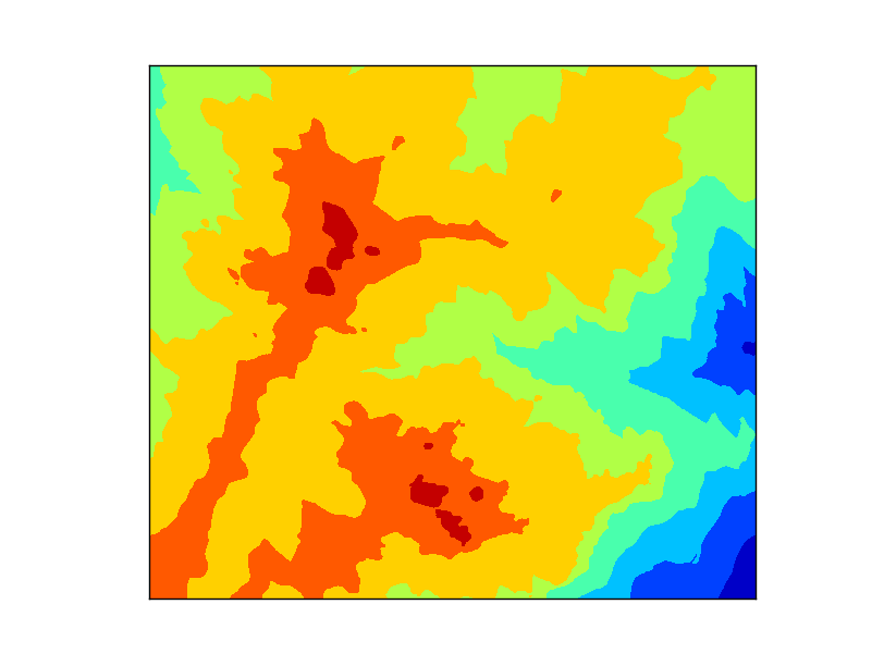
The map is created with the same extension of the raster file, to make things easier.
Before plotting the contour, two matrices have to be created, containing the positions of the x and y coordinates for each point in the data matrix.
- linspace is a numpy function that creates an array from an initial value to an end value with n elements. In this case, the map coordinates go from 0 to map.urcrnrx or map.urcrnry, and have the same size that the data array data.shape[1] and data.shape[0]
- meshgrid is a numpy function that take two arrays and create a matrix with them. This is what we need, since the x coordinates repeat in every column, and the y in every line
The contourf method will take the x, y and data matrices and plot them in the default colormap, called jet, and an automatic number of levels
The number of levels can be defined after the data array, as you can see at the section contour. This can be done in two ways
- An integer indicating the number of levels. The extreme values of the data array will indicate the extremes of the color scale
- A list with the values for each level. The range function is useful to set them i.e. range(0, 3000, 100) to set a level each 100 units

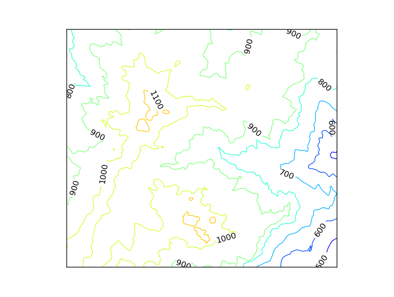
contour¶

from mpl_toolkits.basemap import Basemap
import matplotlib.pyplot as plt
from osgeo import gdal
from numpy import linspace
from numpy import meshgrid

map = Basemap(projection='tmerc', 
              lat_0=0, lon_0=3,
              llcrnrlon=1.819757266426611, 
              llcrnrlat=41.583851612359275, 
              urcrnrlon=1.841589961763497, 
              urcrnrlat=41.598674173123)

ds = gdal.Open("../sample_files/dem.tiff")
data = ds.ReadAsArray()

x = linspace(0, map.urcrnrx, data.shape[1])
y = linspace(0, map.urcrnry, data.shape[0])

xx, yy = meshgrid(x, y)

cs = map.contour(xx, yy, data, range(400, 1500, 100), cmap = plt.cm.cubehelix)
plt.clabel(cs, inline=True, fmt='%1.0f', fontsize=12, colors='k')

plt.show()

The data must be prepared as in the contourf case
The levels are set using the range function. We are dealing with altitude, so from 400 m to 1400 m , a contour line is created each 100 m
The colormap is not the default jet. This is done by passing to the cmap argument the cubehelix colormap
The labels can be set to the contour method (but not to contourf)
- inline makes the contour line under the line to be removed
- fmt formats the number
- fontsize sets the size of the label font
- colors sets the color of the label. By default, is the same as the contour line

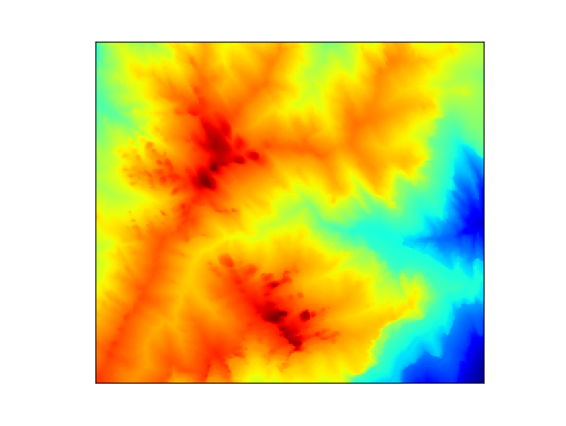
pcolormesh¶

from mpl_toolkits.basemap import Basemap
import matplotlib.pyplot as plt
from osgeo import gdal
from numpy import linspace
from numpy import meshgrid

map = Basemap(projection='tmerc', 
              lat_0=0, lon_0=3,
              llcrnrlon=1.819757266426611, 
              llcrnrlat=41.583851612359275, 
              urcrnrlon=1.841589961763497, 
              urcrnrlat=41.598674173123)

ds = gdal.Open("../sample_files/dem.tiff")
data = ds.ReadAsArray()

x = linspace(0, map.urcrnrx, data.shape[1])
y = linspace(0, map.urcrnry, data.shape[0])

xx, yy = meshgrid(x, y)

map.pcolormesh(xx, yy, data)

plt.show()

The data must be prepared as in the contourf case
The colormap can be changed as in the contour example

Note

pcolor and pcolormesh are very similar. You can see a good explanation here

Calculating the position of a point on the map¶

from mpl_toolkits.basemap import Basemap
import matplotlib.pyplot as plt

map = Basemap(projection='aeqd', lon_0 = 10, lat_0 = 50)

print map(10, 50)
print map(20015077.3712, 20015077.3712, inverse=True)

The output will be:

(20015077.3712, 20015077.3712) (10.000000000000002, 50.000000000000014)

When inverse is False, the input is a point in longitude and latitude, and the output is the point in the map coordinates. When inverse is True, the behavior is the opposite.